本文根据matlab 帮助进行加工,根据matlab 帮助上的例子,帮助更好的理解一维偏微分方程的pdepe 函数解法,主要加工在于程序的注释上。 Ex amples Ex ample 1. This example illustrates the straightforward formulation, computation, and plotting of the solution of a single PDE. This equation holds on an interval for times . The PDE satisfies the initial condition and boundary conditions It is convenient to use subfunctions to place all the functions required by pdepe in a single function. function pdex1 m = 0; x = linspace(0,1,20); %linspace(x1,x2,N)linspace是Matlab中的一个指令,用于产生x1,x2之间的N点行矢量。 %其中x1、x2、N分别为起始值、终止值、元素个数。若缺省N,默认点数为100 t = linspace(0,2,5); sol = pdepe(m,@pdex1pde,@pdex1ic,@pdex1bc,x,t); % Extract the first solution component as u. 
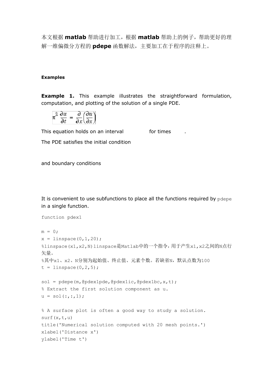
u = sol(:,:,1); % A surface plot is often a good way to study a solution. surf(x,t,u) title('Numerical solution computed with 20 mesh points.') xlabel('Distance x') ylabel('Time t') % A solution profile can also be illuminating. figure plot(x,u(end,:)) title('Solution at t = 2') xlabel('Distance x') ylabel('u(x,2)') % -------------------------------------------------------------- function [c,f,s] = pdex1pde(x,t,u,DuDx) c = pi^2; f = DuDx; s = 0; % -------------------------------------------------------------- function u0 = pdex1ic(x) u0 = sin(pi*x); % -------------------------------------------------------------- function [pl,ql,pr,qr] = pdex1bc(xl,ul,xr,ur,t) pl = ul; ql = 0; pr = pi * exp(-t); qr = 1; In this example, the PDE, initial condition, and boundary conditions are coded in subfunctions pdex1pde, pdex1ic, and pdex1bc. The surface plot shows the behavior of the solution. The follow ing plot show s the solution profile at the final value of t (i.e., t = 2). 我们再将...