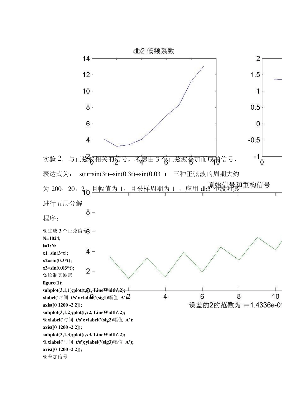
《小波分析》课程结束报告 一.实验目的:运用MATLAB 软件实现一些小波分析的应用,并对小波分析有进一步了解。 二.实验步骤: 实验1.单尺度一维小波逆变换,利用idw t 命令使用指定的小波(‘w name’)或者小波重构滤波器(Lo_R 和 Hi_R)进行单尺度一维重构。 程序: % 当前扩展模式是补零 % 构造原始一维信号 s randn('seed',531316785) s=2+kron(ones(1,8),[1,-1])+((1:16).^2)/32+0.2*randn(1,16); % 使用db2 进行单尺度dwt [ca1,cd1]=dwt(s,'db2'); subplot(221);plot(ca1); title('db2 低频系数'); subplot(222);plot(cd1); title('db2 高频系数'); % 进行单尺度离散小波变换 ss=idwt(ca1,cd1,'db2'); err=norm(ss-s); % 检查重构 subplot(212);plot([s;ss]'); title('原始信号和重构信号'); xlabel(['误差的2 的范数为 =',num2str(err)]) % 对于给定小波,计算两个相关重构滤波器,并直接利用它们进行逆变换 [Lo_R,Hi_R]=wfilers('db2','r'); ss=idwt(ca1,cd1,Lo_R,Hi_R); 结果如下: 实验2.与正弦波相关的信号,考虑由3 个正弦波叠加而成的信号,表达式为: s(t)=sin(3t)+sin(0.3t)+sin(0.03 ) 三种正弦波的周期大约为200,20,2,且幅值为1,且采样周期为1 ,应用 db3 小波对其进行五层分解 程序: %生成3 个正弦信号 N=1024; t=1:N; x1=sin(3*t); x2=sin(0.3*t); x3=sin(0.03*t); %绘制其波形 figure(1); subplot(3,1,1);plot(t,x1,'LineWidth',2); xlabel('时间 t/s');ylabel('(sig1)幅值 A'); axis([0 1200 -2 2]); subplot(3,1,2);plot(t,x2,'LineWidth',2); %xlabel('时间 t/s');ylabel('(sig2)幅值 A'); axis([0 1200 -2 2]); subplot(3,1,3);plot(t,x3,'LineWidth',2); %xlabel('时间 t/s');ylabel('(sig3)幅值 A'); axis([0 1200 -2 2]); %叠加信号 x=x1+x2+x3; figure(2) plot(t,x,'LineWidth',2);xlabel('时间 t/s');ylabel('幅值 A'); %一维小波分解 [c,l]=wavedec(x,5,'db3'); %重构第 1~5 层附近信号 a5=wrcoef('a',c,l,'db3',5); a4=wrcoef('a',c,l,'db3',4); a3=wrcoef('a',c,l,'db3',3); a2=wrcoef('a',c,l,'db3',2); a1=wrcoef('a',c,l,'db3',1); %显示各层逼近信号 figure(3) subplot(5,1,1);plot(a5,'LineWidth',2);ylabel('a5'); subplot(5,1,2);plot(a4,'LineWidth',2);ylabel('a4'); subplot(5...