1、Hilbert边际谱 我觉得既然已经做出 EMD 了,也就是得到了 IMF
这个时候就是做 hilbert 幅值谱,然后对它积分就可以了
程序不是很难搞到吧
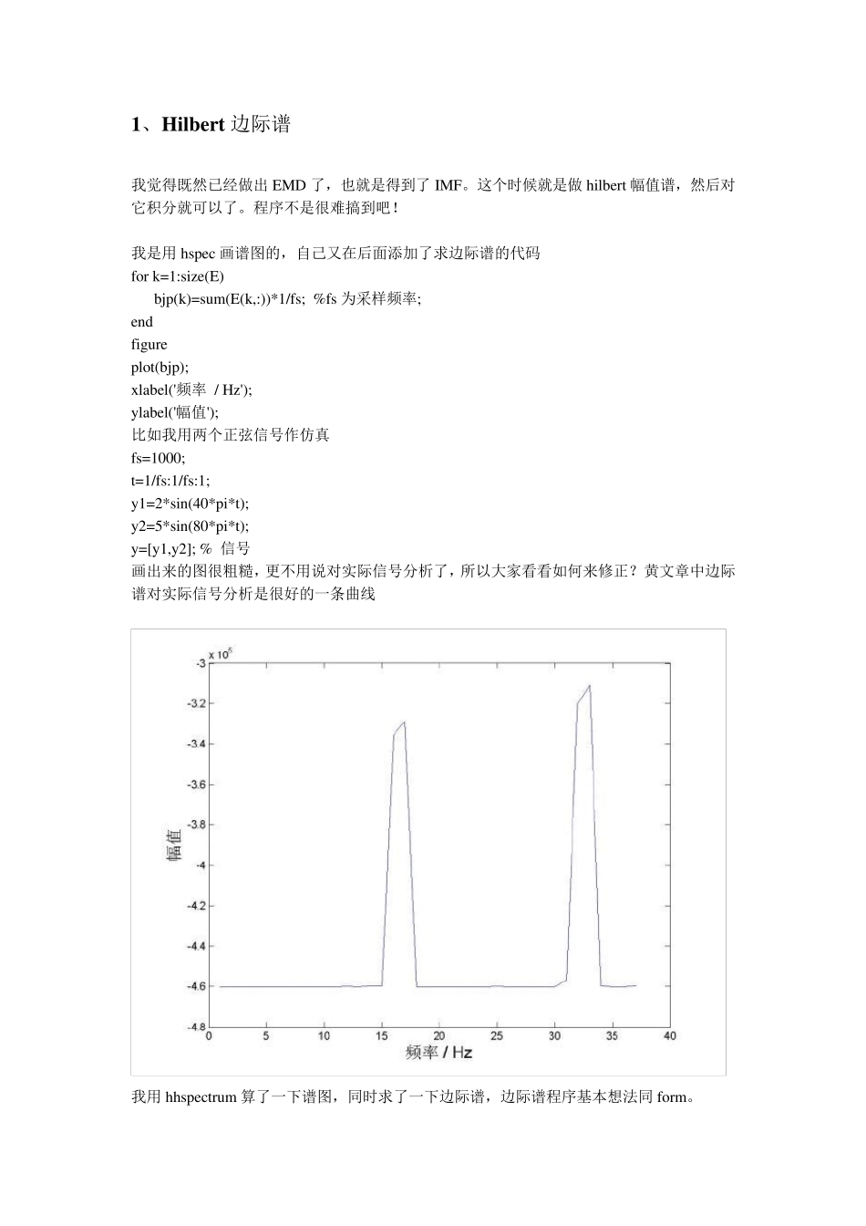
我是用 hspec 画谱图的,自己又在后面添加了求边际谱的代码 for k=1:size(E) bjp(k)=sum(E(k,:))*1/fs; %fs 为采样频率; end figure plot(bjp); xlabel('频率 / Hz'); ylabel('幅值'); 比如我用两个正弦信号作仿真 fs=1000; t=1/fs:1/fs:1; y1=2*sin(40*pi*t); y2=5*sin(80*pi*t); y=[y1,y2]; % 信号 画出来的图很粗糙,更不用说对实际信号分析了,所以大家看看如何来修正
黄文章中边际谱对实际信号分析是很好的一条曲线 我用 hhspectrum 算了一下谱图,同时求了一下边际谱,边际谱程序基本想法同 form
结果也不太好,20HZ 处还行,40HZ 就有些问题了,见附图 你自己再用这个试试 我没有用 rilling 的 hhspectru m nspab: function h1= nspab(data,nyy,minw,maxw,dt) % The function NSPAB generates a smoothed HHT spectrum of data(n,k) % in time-frequency space, where % n specifies the length of time series, and % k is the number of IMF components
% The frequency-axis range is prefixed
% Negative frequency